Inter AS9 and AS4 Routing

Before we diverted pursuant the issue of redundancy, we were just talking about the passage of knowledge from AS9 to AS3. Until now routing has been done inside the AS but now we are going to process routing outside the AS, thus out of NetByCabo domain. AS9, or the ISP NetByCabo, is typically the case of an ISP that covers all levels from level 2 to the access level.

In the other side o four journey, we considered AS3  completely identical to AS9, with the same number of addresses, the same subdivision, etc.. Only its name changes. We will call it ClientInNet, which will be divided into ClientInNet 1-8, which in turn will be divided into CIN 1.1 to 8.8. Of course, any one of these ISP advertised as 18 bit networks, offering only 2¹⁴=16,384 addresses, defined as ISP level 2, belongs to the realm of imagination, but accomplishes the goal of making better understandable the various aspects related with routing.

Between AS9 and AS4 in our case study, we are going to deliver routing to Level 1 ISP, therefore only delivering Backbone services. This routing process could go through all the imaginable ways, hop-by-hop through the border routers of the various Level 2 ISP (AS), even never using a Level 1 ISP.   All this communication lines are possible and can be used, once the administrators of the several networks, due to technical or commercial policy reasons, give preference to determinate routes, assigning them lower costs and thus diverting routing to them.   As you easily can understand, if we put together in our graphic all those possible lines of Inter AS routing, the graphic would become unreadable, what is far from being our purpose.

Backbone AS – Level 1 ISP – eBGP

AS3, AS1 and AS2 are Backbone ISPs, thus level 1 ISPs.  Through their border routers, the remaining AS pass them the addresses of networks they know and undertake to deliver. These network addresses are loaded into the routing tables, which can include other elements, such as AS-PATH or NEXT-HOP.

• AS-PATH is made up of all the AS IDs that are traversed, until you reach the border router that passes the information to the AS  to which the router who’s filling the table belongs . Each time an AS passes the information to another AS, it includes its ID in AS-PATH.
• NEXT-HOP router, is used by the router filling the table to record the address of the router that provides it a certain information. When passing that information, the NEXT-HOP router is giving the gateway address in case its information is chosen. Another route to the same destination may have been announced by another NEXT-HOP router. Thus, the receiving router can identify the router that gave him the chosen path and associate it as the gateway for the interface that links to it. Let’s remember that each router in its routing table stores only one route to each destination.

The path between two  routers is always made through HOP-by-HOP routing. HOP-by-HOP routing is one of the main features of Internet  network layer in contrast with end to end transport layer connection. Since router tables are consistent with each other, delivering HOP-by-HOP , thus always delivering to NEXT-HOP, ensures arrival at destination. Tables consistency and defense against routing loops, were some of the innovations brought by BGP.

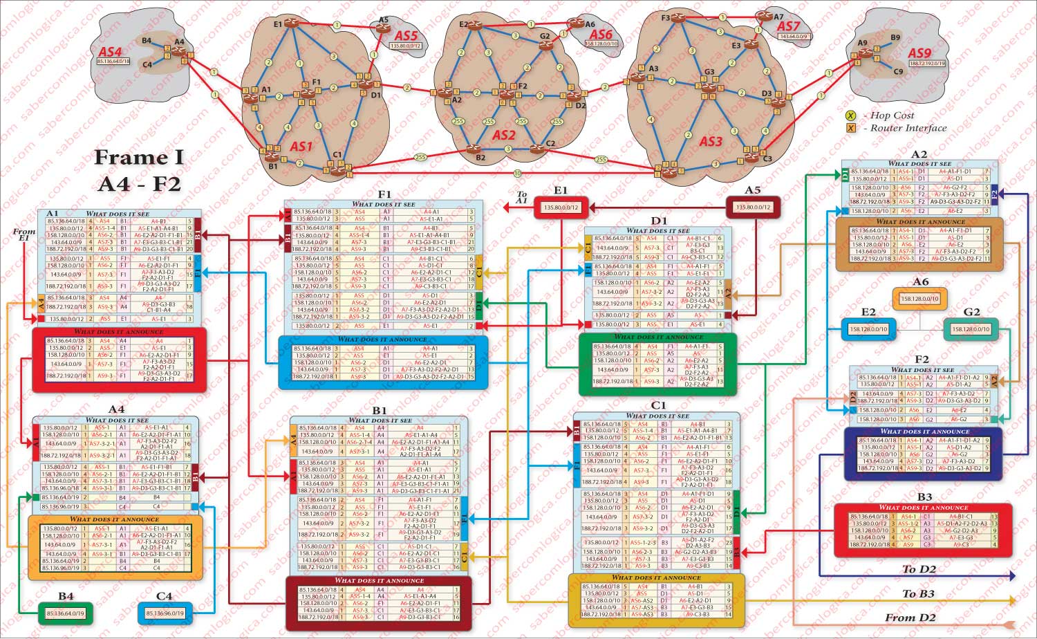
Our goal now is to understand how the border router A(AS9), for which we already understood how it can get us to our destination, manages to convey this information to the border router A(AS4), where lives the client requesting a page lying in the server who’s in AS9. It’s through BGP that it will happen, that we already know, but in order to better understand how BGP makes it happen, we decided to add a chart based on links between AS4 and AS9 in Figure 1 of the previous articles (whose insertion we are not going to repeat in this article), building frames representing all routers in two basic chosen routes, illustrating how each one receives the information of its neighbors and builds its routing table which in turn it announces to the same neighbors.

Because this table doesn’t fit into one figure, it is shown in Figures 1 and 2. Relatively to them we say the same thing we said to figure 1 of previous articles: If you want to follow the description having them in presence, you must open them in a new window. For easier reading and interpretation of the tables included in the figures above, we added also a caption for them in Figure 3, that soon we will describe, just after we formulate some presuppositions we assumed for those frames preparation.

 We assumed that we would only integrate in the construction of the tables the routers of two basic routes defined by AS-PATH AS4-AS1-AS2-AS3-AS9 and by AS-PATH AS4-AS1-AS3-AS9, though we will integrate the information they receive about the networks present in AS5, AS6 and AS7. Therefore we assumed that the routers E1, E2, F2, F3 and E3 (notice the new routers designation, accordingly with the new graphics) are not analyzed, contributing to the set solely with the information that each one provides about the way to AS5, AS6 and AS7. Routers B2 and C2 are not included in the construction of tables too. With that propose, the cost of each of the links between them and the remaining set is elevated to 255, what matches the effect of traffic interdiction in each of them.

Choosing a Route

In BGP, each router only allows the existence of a single route for each subnet, which is chosen among all possible it is advertised by its neighbors, by a criterion that favors the cost of the route. ISP network administrators usually assign costs to links as a way to make certain pathways favored over others. This is the method of allocation of costs to a path by learning from neighbors. Those who transmit the cost of the announced routes to destination will in turn learn that same cost from their neighbors, and so on.

The cost assigned to a link goes from 0 to 255, corresponding 255 to a prohibited traffic signal. The allocation of costs to different links for each ISP is done manually by network administrators of that ISP. Parameters such as the reliability and other filtering criteria preestablished, are taken into account in establishing these metrics. Network administrators of an ISP can also assign direct costs to a route in a given router, for it to be preferential or rejected. It is important to note that in choosing a route influence trade policy issues between the various ISP acting in that route, what turns necessary the method now stated. In this method the router does not learn through others but for himself, and thus ignores the information others provide for the cost.

The best route to the same destination may differ from router to router, depending on the possibilities that its neighbors announce and on its choice. What is certain is that in each router the chosen route and therefore the announced one is always the best possible:

• The lower cost one, or in case their cost is equal
• the lower AS-PATH one, or if yet equal
• the lower cost NEXT-HOP router

During the construction of the tables for our case study, several of these options will be checked.

The Routing Table and its Caption

All routers in backbone areas involved in BGP are aware of the best path for each of the AS announced to BGP routers.
AS4, AS5, AS6, AS7 and AS9 are supposed to be level 2 ISP that provide access services, transmitting to their backbone regions information about their knowledge.
Therefore, the routing tables of all routers that will be considered in our work will have the information provided by those areas in its tables. But, as already stated, the paths set out by each of them may be different, depending on the rules and values ​​that are communicated.

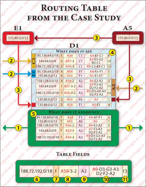
Thus, we decided to affect each router with a table as the example in Figure 3 where we can see two distinct zones and some informations:

• Zone 4, containing the values transmitted by each of the neighbors, grouped in blocks and provided with a label identifying the transmitting neighbor.
• Zone 5, containing the values ​​chosen  according to the above described rules, which shall be announced to all its neighbors. Zone 5 represents the routing table of a router. The routing table is represented within an area identified and highlighted with different colors for each of the routers on the board.
• The informations received by a router and marked with 2 match the individualized blocks provided by routers who have their own routing tables, which are described in the figures.
• The information marked with 3 comes from routers that are not included in the preparation of tables, intervening only with an indication of the networks that they announce.
• The arrows marked with 1 indicate the direction of propagation of information, i.e., the routing table which is brought to the attention of the neighbors.

A router ignores the information that is supplied by another which corresponds to the one provided by itself. This happens when the chosen route to a destiny in one neighbor router is the one provided by it, therefore included in its routing table and announced to all neighbors, including the provider. This kind of loop is easy to avoid, just checking that the indicated route is the same it provided having itself as NEXT-HOP. But the actual cause of endless loops is the result of information that has already been passed by a border router from an AS and comes back to this same AS through another border router of this AS. To avoid this, BGP has a property that allows a router to reject information which already includes in AS-PATH its own AS.

The Routing Table fields are as follows:

• Field 6 refers the destination subnet address of the  route indicated by this table row.
• Field 7 indicates the router interface that connects to NEXT-HOP router.
• Field 8 indicates the AS-PATH route announced. In the example it indicates that the announced route was sent by a border router of AS9 to AS3, then sent by AS3 to AS2, and finally from this last one to the current AS. Its AS ID is not part of the AS-PATH. The AS ID is included in AS-PATH by any AS when the information is passed to another AS. If AS1 was part of the AS-PATH, we were facing an endless loop, the announced route being discarded, according to the already stated BGP property.
• Field 9 identifies the address of  NEXT-HOP router, here represented by its ID (letter and AS number). It is the gateway for the indicated interface.
• Field 10 matches HOP-by-HOP registration, i.e. the hops  performed by this route till this router. This element is not usually part of the routing tables,  but we included it in order to enable a better understanding of what each router sees and announces. The criterion used for its formation was identical to that used for the AS-PATH, i.e. each router that passes the information includes its ID in HOP-by-HOP registration.
• Field 11 indicates the total cost of the announced route from this router to destination.

Creation of Routing Tables

All routers involved in BGP routing are aware of the same sub-networks and their preferential routes for them. But, for each one such route is different.

How does the border router A1 from AS1 learn the routes that the border router D3 from AS3 announces and vice versa?

The answer to this question lies precisely in the Routing Tables way of creation. First we must understand the scope of such a statement. A border router of an AS matching a level 2 ISP in Australia knows the same subnets that a border router of an AS matching a level 2 ISP in Portugal. This means that all the networks announced by BGP backbone border routers are known to all routers under BGP. The result of this statement are routing tables with hundreds of thousands of entries, despite only being announced network addresses, meaning CIDRized addresses, aggregated always that it is possible.

Information on the knowledge of the Portuguese ISP border router is passed to its neighbors and so on, HOP-by-HOP, until it reaches the Australian ISP border router. Likewise the  information of the Australian ISP border router arrives to the Portuguese ISP border router. Along the way both will collect information from other destinations to whom they pass their ones. When we say that the routing tables have hundreds of thousands of entries, we mean that there are hundreds of thousands of information entries coming from each one of a router’s neighbors, from which it chooses its preferred for each announced route, including it in its routing table. Then it passes to all its neighbors the hundreds of thousands information entries of its table, but now under its point of view.

As you can see, this results in a monstrous interconnection that must be equilibrated and stable until it leads to the routing table of each router. Enormous complexity, always dinamic and in permanent actualization. One router which is conected or disconnected, a new subnet which is announced, are enough to generate a huge information movement. Fortunately only the updated information is passed by each router to its neighbors.
We think now you will understand why we have limited the number of routers that are part of the creation of the routing tables of our example. Only routers that have marked the number of their interfaces in each link are part of the network contributing to table’s creation. And even being only for those, it took four pages to accommodate the resulting information in a perceptive manner.

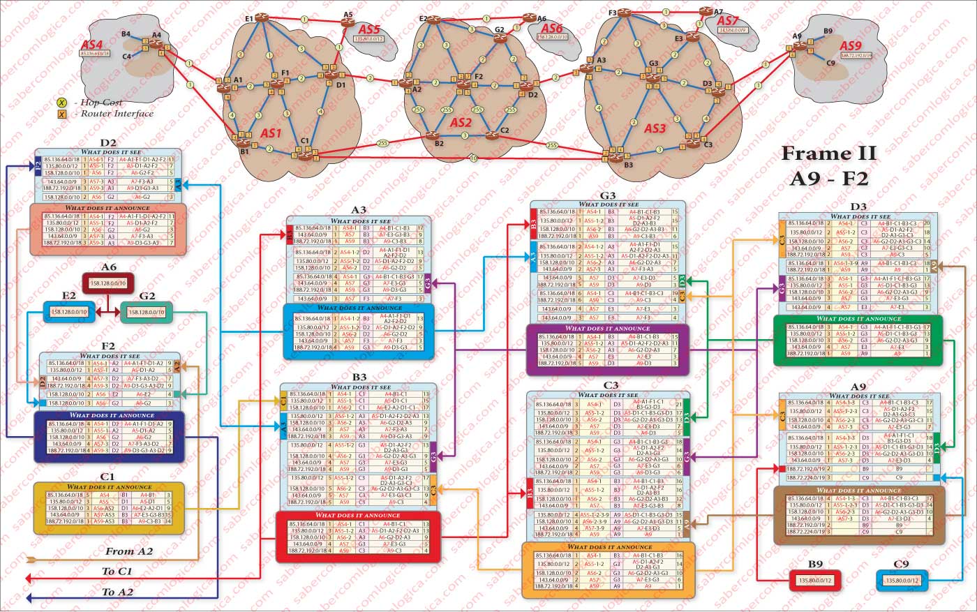
It is our goal to understand how it works. For this purpose nothing better then to make it work, but on a scale as small as possible, so that dispersion and vastness don’t lead to the opposite effect. It’s irrelevant the side from which we start (AS4 or AS9), because at the end all tables will have to met each other before the information is complete. So let’s start by both sides, spreading to the center the information that is collected in each of the paths. Once there, each one transmits to the other the information gathered in the meantime. Then its time for each one to return to its starting point propagating the new acquired information. This separation is reflected in the two tables of  figure 1 (from SA4 to SA2) and from figure 2 (from SA9 to SA2). But, in the tables of both figures is already reflected all the final information of each table.

Let’s begin by assigning costs to all links and number the router interfaces that will be part of the creation of the routing tables. Now let’s look at router A9 routing table. As we can see in its actual presentation, it already sees the information of neighbor routers about all the network and has on its table the chosen routes for all announced subnets. But let’s start by admitting that none of this information is there. Only the information that comes from its AS Areas is known for now and will be announced to the neighbors C3 and D3 from AS3. Thus, in these last routers we must write blocks relating to the information they see in router A9 , now in an aggregate manner.

Now, routers C3 and D3 are also announcing their own routes to A9. But D3 sees C3 and C3 sees D3. Thus we must  fill in each one the blocks in which the information he receives from the other is displayed, with the route each one sees in the other. But not announcing them on the table, for both they have a better route to the A9. D3 also sees E3 and through it A7. Thus we must register in the adequate interface information block the information that is provided by E3, which will be unique in the block and definitive, because E3 will not have a routing table in our case study. This information will be passed to D3 table and consequently for C3 table. In the meanwhile, the information from both D3 and C3 tables is visible to G3 and B3 and must be registered in their respective display. But G3 sees B3, A3, E3 and F3. The information that they transmit will be recorded in the appropriate locations in G3, the best route for each one will be chosen and registered in its routing table.

And so on, always running all the information through all neighbors, adding or correcting the information of those who were left behind and propagating it if its the case. Soon we will get to what we will define as the virtual boundary between the two paths:

• The routes which come from A4 will have virtual boundary in A2 and C1.
• The routes which come from A9 will have virtual boundary in D2 and B3.

A2 and D2 transmit their information respectively from A4 and A9 sides to F2, who in turn collects the information transmitted from both opposite sides, chooses the best route to A6 and propagates the new information the way up to A4 and A9 through A2 and B2 respectively. C1 and B3 exchange information among themselves and then propagate it the way up to A4 and A9 respectively.

We are certainly not going to describe how the whole table was constructed step by step. We have described the essential about the strategy to do that, always bearing in mind the need to maintain consistency across all tables. This means that each router always has to see all the information of neighbors, even though it may seem pointless, in order to make the right decision. Some more notes:

Note for example that C1 sees A5 and A6 all the way around through B3 and SA2, as we can see in zone 4 of its construction table. Its enough to change the metrics of some links of C1 for this to be its preferred route to those routers.

Note how B1 chooses the best path to A7 between two metrics with the same value, just by choosing one with the smaller AS-PATH.

Note that the preferred route from B1 to A5 is through A4. Only when that route has been registered in the table of A4 and spread to the table of B1, it has been possible to define it as B1 preferred route to A5, registering it in B1 routing table. Before that, B1 had a different preferred route to A5, all inside AS1.

Suppose that AS1 ISP has not permission to cross AS4 with information that is not designated to it, maybe because it has not negotiate that permission yet. Thus, AS1 ISP administrator will have to correct the cost of some links in order to avoid it and bearing in mind that any change will affect all the other choices HOP-by-HOP, even those that he doesn’t want to. All these suppositions and some more have to be taken into account during the creation of routing tables, something that in our case study we obviously didn’t do.

We will stay here with this description. We leave you the Figures 1 and 2 with the tables, the tables caption in Figure 3 and the strategy to create the routing tables. Certainly trying to understand  this by making any journey creating the tables, will clarify you a lot more questions than now by writing more about what has already become clear and readable. Therefore we suggest a try.

In the meanwhile, the information about the network where we find the server we were looking for is arrived at the border router of AS4, where the client requesting the page lives.

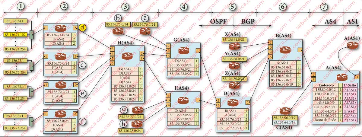
Targeted information through iBGP to the border router of the Area of that client, the same is brought to the Gateway router of its network by OSPF protocol, as shown in  Figure 4. We dispense Further description about this path, since the same would be identical to the already previously made for the opposite trip in AS9. We leave its graphical description in Figure 4

We have just analyzed the main features of network layer, routing and addressing. We have seen how IP protocol does, how to build the datagram header, how an address is assigned and how we find the route to that address.

We are now able to send the datagram to the layer below and go after it.