TCP Recognition Improvements

Because this solution is not satisfying, TCP has undergone several improvements in the way it ensures reliable transmissions.

The Timer

The timer, after a replay because it was exhausted, doubles its size. If it runs out of timer again in the same packet it doubles its size again. And so on, until the packet can be recognized without exhausting the timer. Met the goal, barely passing to the next packet, the timer returns to its value calculated and updated, as usual.

This procedure works now as a primary way of congestion control. If a package is not recognized within the period of the timer is most likely because the network is congested. By delaying the retransmission of packets TCP avoids further congesting the network.

SACK (Selective ACKnowledgment)

Another modification is the introduction of SACK. Selective ACKnowledgment is the ability of the recipient to recognize packets, regardless of whether they come or not in order, simply looking to its integrity.

Thus, the recipient shall be able to have in its reception window packets received and acknowledged having gaps between them, as does the window of the sender.

How does the sender know that there is a gap?

Now TCP, whenever a packet is received out of order but in good condition, an acknowledgment for the packet and an acknowledgment for the last packet received in order is sent to the sender, thus maintaining the same negative acknowledgment procedure regarding the sender for the last packet received by the appropriate order, that it musts repeat after three ACKs.

How does TCP send two ACKs simultaneously?

SACK, widely used and accepted by almost all implementations of TCP, has to be negotiated between the sender and receiver terminals (Browser and Web Server). Such trading is done during the 3 way handshake in section header options.

The header options! That’s it.

Yeah, that‘s it. It’s indeed the way TCP solves its problem. It sends an acknowledgment for the last packet received in the order and in the header options it sends a SACK with initial and final numbers of each sequential set of packets that it has already received out of order. Thus, the sender learns that there is no need to resend those packets.

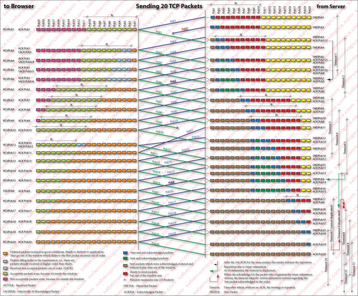
Some of these steps can be followed in Figure 1, which we are going to comment (click or touch the figure and open it in a separate window):

Sending 20 TCP packets from the Web Server to the Browser is the topic. The agreed reception window is for 10 packets, value that remains constant during the session. It was also agreed the use of SACK.

Packet 2 is lost during shipment. Upon receiving the package 3, the browser sends an ACK for the packet 1 (the last received in order) and a SACK denouncing the acceptance of packet 3. It proceeds similarly to the packets 4, 5 and 6.

Upon receiving the 3rd ACK for the packet 1, the server resends the packet 2. When the browser receives it , sends an ACK to the server and slides the window to the end of the last packet received in order. The now ordered packets 1, 2, 3, 4, 5 and 6 leave the window and are ready to be delivered to the application.

On the server side, when the ACK for packet 2 is received, it slides the reception window and restarts the timeout from the last packet received in order.

Each time a packet is received in the correct order timeout is restarted and placed ahead that package. Hence the appearance of numbers after the timeout. It’s intended to illustrate their version.

The ACK for packet 9 is lost. The browser has no way of knowing it, because the server expects it delayed and out of order. Nothing tells it that the packet has not been delivered. So, it will only resend the packet when the timeout is exhausted. In this case, the timeout is restarted at the same point by double the amount.

Browser will receive packet 9 again, but dismisses it and sends an ACK. Otherwise server would never slide its window resending packet 9 after the exhaustion of each timeout. When the ACK for this packet reaches the server timeout restarts from that point with its normal value.

There is also a slight advance of packet 11 and a slight delay of packet 12, which leads to the fact that they arrive out of order. When packet 12 reaches the browser it lacks packet 11. Thus, it sends an ACK to packet 10 (the last packet arrived in order) and a SACK for packet 12. As soon as packet 11 reaches the browser it sends an ACK for it instead of issuing another ACK for packet 10.

The server, as it didn’t received the ACK for packet 10 in triplicate, doesn’t repeat packet 11, considering he was received by the browser.

Both are still adjusting their windows and timeout until they complete the transmission.

TCP Congestion Control

Network’s congestion is one of the main causes of propagation delays. And it can happen on any link of the route that packet follows till the recipient.

We are going to involve some concepts that are only worked in the Network Layer, but which are necessary to understand what we are going to analyze.

So, when a packet travels from a sender to a recipient, it doesn’t follow a straight path, i.e. it is not like an high speed train, being more like a mail train, which stops in all stations in the route.

Do you remember the little cars carrying the leaves of our message? In their path they will find many intersections (the mail train stations) and roads of different sizes and speeds. When they reach an intersection they need to know which road to follow. So at every intersection there is a signalman, which we call the Router.

The roads between our computer and the first signalman, between the different signalmen that the little cars will find in every intersection along their path and between the last signalman and the recipient, are called links.

Different roads (links) will have different capacities, and signalmen in the intersections will be more or less efficient.

Just like some little cars depart from our computer, many others leave from other computers and many of them will get at the same intersections in the path to their destinations.

If the cars driven by signalmen and sent to the same intersection exit road, are more than the flow capacity of that road, they will generate what we call a traffic jam. TCP calls it congestion.

How does TCP know all intersections and roads that go, for instance from Lisbon to Paris? And even if they have and where they have congestions?

It doesn’t! Therefore it uses alternative methods that allow it to assume whether or not there is a congestion on the path in order to be able to prevent it.

This is where the window reception, which so far we have pointed only for control flow, will play a fundamental role. It will be through the window size that TCP will set the number of packets laying on the network simultaneously.

Let’s see how.

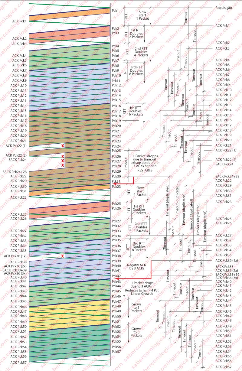
We will use Figure 2 to follow the analysis.

Let’s begin by considering a variable CW (Congestion Window) which matches at each moment the size of the window.

When sending a message, a set of segments, TCP starts in a way that has come to be appointed as Slow Start.

In Slow Start, the window size CW, begins with the MSS size, i.e. the size of a segment. On receipt of the first acknowledgment, i.e. after an RTT (Round Trip Time) TCP doubles the size of CW (in this case to 2 MSS). When receiving each one of the sequent ACKs, TCP is back to double the size of CW (4 MSS, immediately afterwards 8 MSS, and so on). CW will be on exponential growth until it receives a first sign of packet loss.

TCP recognizes the loss of a packet by timer exhaustion or by the reception of 3 ACKs for the same packet. From now on both situations will be referred as packet loss.

When this happens, TCP starts by determining the value corresponding to half the value of CW at that moment and creates a new variable TR (ThReshold). From now on TCP will have two distinct types of behavior, depending on the situation that caused the failure:

• If the cause was timer exhaustion, it reboots a slow start, by doubling the value of CW until it reaches the value of TR. Thereafter it shall proceed with a linear growth of CW, by adding to CW one MSS value for each received ACK, until it receives a signal of packet loss.
• If it has received 3 ACKs for the same package, reduces the size of CW to the value of TR and thereafter starts with a linear growth of CW, by adding to CW one MSS value for each received ACK, until it receives a signal of packet loss.

TR value is dynamic and is fixed each time a packet loss indication is received.

But why at every indication of a packet loss?

The loss of a packet results in most cases from congestion. When a router has in one of its incoming links, a queue that exceeds a certain number of packets, it simply drops the surplus.

Packet loss signal indicates a most likely congestion in an intersection in the path to the recipient. Thus TCP proceeds accordingly, reducing the number of packets that releases in the network. As all TCP accessing this intersection will do the same, congestion will effectively be reduced allowing the normalization of traffic.

It would be great if at all intersections that we have to cross to access our destination every morning or afternoon ,there were a signalmen who in case of traffic jam should call all settlements that cause traffic to that intersection to indicate that traffic should be reduced. Certainly all we would arrive a lot faster at our destinations.

And why different reactions to different situations?

Properly understood, we will realize the difference of the different reactions.

• If the sender receives 3 ACKs for the same package is because two other packets after that one went through. Congestion reduction doesn’t have to be drastic. It reduces CW to TR and goes forward slowly. It enters the congestion avoidance state.
• If the sender receives an indication of timer exhaustion, it’s because none of the other packages went through. The congestion must be severe, thus demanding a drastic solution. It reboots a slow start and only after TR enters is the congestion avoidance state.

Why both exponential and linear growth?

If the sender did early adopt linear growth for CW, transmission would become probably unnecessarily slow. Thus, starting with an exponential growth of CW, it will quickly grow and TCP can quickly realize the state of network congestion. So, it can certainly better strike the value from which growth will be linear (TR).

Congestion control suffered a major evolution with the implementation of the ECE and CWR flags, which together implement a process of congestion control, the ECN (Explicit Congestion Notification).

To talk about this method, once again we’ll have to move forward .

Because this process of congestion control, aims to avoid dropping packets in a queue of a router, this router has to mark them with an indication of congestion. Here we will have a problem. The router does not open the package to the Transport Layer. It only opens it to the Network Layer, where prevails the IP protocol, not yet mentioned. Therefore, its mark must be included in this protocol, by the completion of two bits that indicate:

00 – Does not support ECN
10 – Supports ECN
01 – Supports ECN (for servers)
11 – CE (Congestion Encountered)

When sending a packet, the sender marks it with 01 or 10 (as it is a server or not)if it supports ECN and the Router with congestion marks it with CE (11).

Upon reaching the recipient, the package opened in the network layer indicates congestion, being this information passed to the upper layers where the recipient, when filling TCP header sets ECE (or ECN – Echo) flag, i.e. echoes to the sender a congestion signal in TCP.

When the sender receives this packet, it reduces the size of CW as if it were a loss and sets the flag CWR (Congestion Window Reduced). Until the recipient receives this packet with the CWR set, it continues to send packets with the ECE flag set.

This process works only on routers that use AQM (Active Queue Management ) and RED (Random Early Detection). In these cases, routers can, at the expense of algorithms that make analysis of changes in the traffic, predict in advance that the buffer an input interface will saturate and then, marking packets with ECN before it happens, they avoid dropping packets as TCP way of synchronization.

Support for TCP ECN is implemented in versions Windows 7 and Server 2008 (by default off) and in recent versions of Linux and Mac OS X 10.5 and 10.6.

The full use of this method, which effectively makes the transmission of messages more efficiently and quickly, requires that all actors of the process were ECN Capable.

The use of ECN is optional and its use must be negotiated between the terminals through the messages of presentation options.

Well, we are now able to send the packets to the network layer, which will deal with its address and routing.

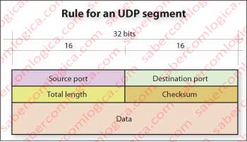
But first let’s see the rule for a UDP (User Datagram Protocol) segment, represented in Figure 3.

Source port, destination port and checksum have the same meaning as in the TCP segment. Total length is the length of the segment, including header, in bytes.

We’ve done some considerations about UDP and what kind of applications do use it. Query applications such as DHCP and DNS also use UDP.