Digital Image Types

Do you remember when, in the beginning of this Chapter, we used a powerful lens to approach the screen in order to see the image in more detail? Why approach the screen and amplify it with a lens, instead of simply zooming in the image?

The answer to this question has to do with the image type, and with the difference between the composition of a display screen, and that of an image. Both of them are composed by pixels.

Since in the previously described situation, we wanted to see the screen’s structural detail, we had to approach by using a lens.

If we wanted to see the image’s structural detail, then we should have to zoom it, but we would only succeed if we were dealing with a pixilated image. If it would have been a vectorial image, as was the case, we would have not succeeded, because we would always get a defined image.

So, it’s better to begin with the analysis of the different types of image before going into any further explanations.

Vectorial Image

Vectorial Image is an image composed by straight and curved lines, drawn in a graphic design program, such as AutoCad, Illustrator or Express Blend, for instance. These lines may or may not form enclosed areas.

This type of image is obtained by the mathematical calculation of the functions that represent each of the lines, and being rasterized afterwards to a pixelated structure, identical to the one in the screen where it’s going to be printed, meaning one image pixel per screen pixel. Each time we zoom, the image will be recalculated for its new appearance and rasterized again for the pixel structure of the screen.

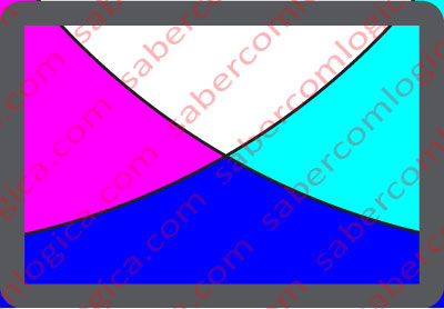
Meaning by this that, in the previously described situation, if we had zoomed in, the resulting image would have the appearance of the one in Figure 1. The display’s pixel structure wouldn’t be visible (at the same distance and with no amplification) and the vectorial image would be perfectly adapted to fit that structure.

As we said, a vectorial image results of mathematical calculations. So, we believe it’s important to briefly mention what Mathematics as to do with it. It will only be a slight approach. Anyway, we recommend that those who are not interested in Mathematics jump directly to the end of this section.

A few lines ago we mentioned a function, didn’t we?

Function is one of the most important concepts in Mathematics. The function f(x) establishes a mathematical relationship, in which, for each value of x, there is only one value of f(x). This value will be calculated by the expression that includes x as a variable, and is associated to f (x). For example:

f(x) = 2x + 1  or  f(x) = 5x/2 – 5

are examples of linear functions, and

f(x) = x² + 3  or  f(x) = 3x²/5 + 3x/2 + 3

are examples of quadratic functions.

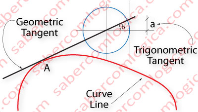
The execution of a function f(x) with several values of x returns a straight or curve line, whether the function is linear or quadratic. The curved line of Figure 2 is certainly defined by a quadratic function.

That curved line, or function of x, has at each one of its points (ex. at point A) one tangent line, meaning a straight line that touches the curve only in that point, or rather, its geometric tangent in that point.

To this geometric tangent corresponds the value of the trigonometric tangent (a) of the angle between the geometric tangent and the X-axis.

The Derivative of a function at a given point (A) defines the slope of its geometric tangent in that point. The slope of a line can be defined by its angle with the X-axis. And this angle (b) is defined by the value of the trigonometric tangent of the function in that point.

So, if we know the value of the trigonometric tangent at a given point of a function, we will also know the slope of its geometric tangent at that point. The Derivative of a function at a given point represents the function’s instantaneous rate of variation in that point.

For instance, the derivative at a given point of a function that represents the speed of an object (speed in Y-axis and time in X-axis) represents its instantaneous acceleration, or speed variation, in that point.

When the derivative of a function at a given point is equal to 0, it’s because the trigonometric tangent of the function at that point is 0, thus the geometric tangent at that point is parallel to the X-axis.

At that point, the function will have a maximum (increases before it and decreases after it) or a minimum (decreases before it and increases after it), but its instantaneous rate of variation at that point is 0.

In the case of our previous example, the acceleration of the object at that point would be 0, meaning its speed would be constant, without variation.

And here it is, how functions, derivatives and trigonometric tangents can be used to define a line.

How does this help us? How can we visualize this in practical situations?

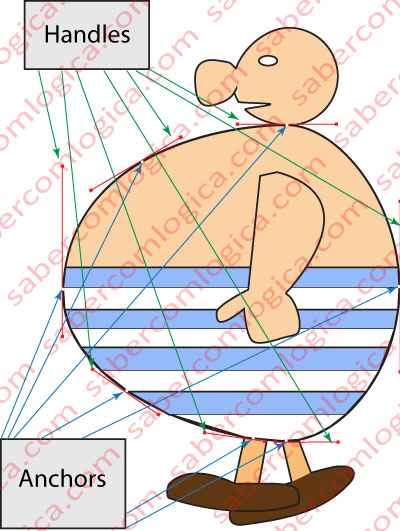
Well, this is where a vectorial graphic program will become useful for us. With it, we can draw any image within a computer. As an attempt to illustrate a practical situation, we developed with the help of a vectorial graphic design program, Adobe Illustrator, a representation of Obélix (any resemblance to reality is pure coincidence) that we present to you in Figure 3.

Then we highlighted the body line building elements. Notice the red Handles, connected to the white dots that show up along the curved line of the body, also known as the Anchors. The green arrows point to the Handles, while the blue ones point to the Anchors.

The Anchor points, as the name says, are the starting points (or anchors) of the functions which define the line starting from that point. One on each side, given that handles can be used to define an angle at that point. This is not the case in our example, to facilitate matters.

The Handles define the tangents to Obélix body curve, in specific points. The Handles length define a bigger or smaller variation in the trigonometric tangent value, until the next anchor point which, in turn, has the same definitions.

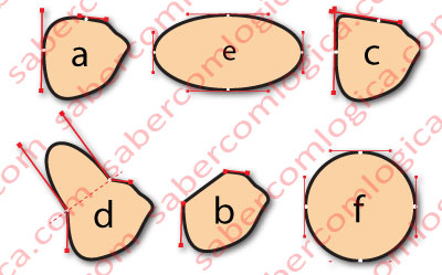
In Figure 4, we purposefully made changes to Obélix nose Handles. a represents its original shape (in Obélix image, we can’t see the part of the nose that is hidden by the face).

• a. Here we can see the Handles of the two most left Anchors, as they were in the original representation.
• b. We reduced the Handles that go from the Anchors to the tip of the nose to 0, resulting in a linear function between those two Anchors. The derivative, or geometric tangent slope, at any point between those two points will be constant. In our previous example, the acceleration would be constant between those two points.
• c. We extended the Handle that goes from the upper Anchor to the tip of the nose to a similar to the one of the lower Anchor, thus reducing the tangent’s rate variation from that point on. The variations of the tangents to the lines which go from both Anchors to the tip of the nose are now similar, and low. This way, in the middle points, the line makes a strong revolution in order to unite both lines.
• d. We broke the Handles which converge to each Anchor. Then we increased the length and displaced the Handles facing the tip of the nose, leaving them perpendicular to an imaginary line (a dashed line) joining the two points and giving them the same length. The result is a half ellipse at the tip of the nose. An ellipse which grows as the Handles’ length grows and vice versa.
• e. We created an ellipse in order to understand how the Handles work in that case.
• f. We did the same for a circle.

We will finish here our small approach to Mathematics. Those who jumped this section must resume their reading from here.

Until now, we’ve tried to clarify the influence of mathematical concepts in the calculation of a line’s shape. It’s now time to see how it works with surfaces, even 3D ones.

Find a piece of chicken wire. Hang it by its 4 corners and punch the middle.

What do you get?

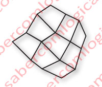
Well, apart from a piece of rumpled chicken wire, we get a curved surface, built by linear vectors that form polygons joined together, as you can see in Figure 5. It’s almost like a Wireframe, where the vectors, which we assume still remain linear, are the pieces of wire between the nodes.

In a real Wireframe, these vectors are mathematically calculated in order to build surfaces (the polygons) which, together with each other, form the 3D image shape. Then, these polygons are filled with textures, which can even be copied from real photos, light effects, shadows, transparencies and others, until we achieve the nowadays magnificent 3D vectorial images present in Games, Buildings, Apartments, Automobiles, and so on, which are sometimes confused with real photos.

The bigger the approximation to reality, the denser the Wireframe will be.

If you want to visualize what we have just described, we recommend that you download and install a free test program called Heaven Benchmark, developed by Unigine, which owns one of the most advanced platforms for 3D image creation. When running this program, you must go to the Settings and in the window that opens up, choose the option Wireframe or, alternatively, press the F2 key. You will then visualize a multiple vector structure, the Wireframe, over the running images, and understand how they are filled.

 So far we’ve referred to Vectorial Images, created within a computer by a huge amount of calculations executed at an incredible speed, let’s say, around 2 billion operations per second, per processor core.

But, for the vectorial image to be seen in a display screen, it must first be rasterized, which means, it must be converted to a pixelized image, an image composed by pixels, with the same number and composition as the screen structure.

Pixelized Image

The pixelized image is composed by pixels, each pixel having only the color information.

Since that information is provided in bits, it sometimes assumes the name of Bitmap, which is the origin of the BMP image format, although JPEG, or JPG formats, are the most common when it comes to compressed images.

We must also mention GIF and PNG as being a few other, very common, image formats.

When we say that a digital camera has a resolution of 5 Mega Pixels, we mean that each photo it takes is composed by 5 million pixels.

In the case of our monitor, who has about 2 million pixels, an image shown at 100% (one image pixel per display pixel) would only be partially visible on the screen. To be able to fully see it on the monitor screen, we would have to zoom it negatively, meaning, prepare it in  such way that about 2.5 of the pixels’ information was converted into 1 pixel information, and then send it to the screen.

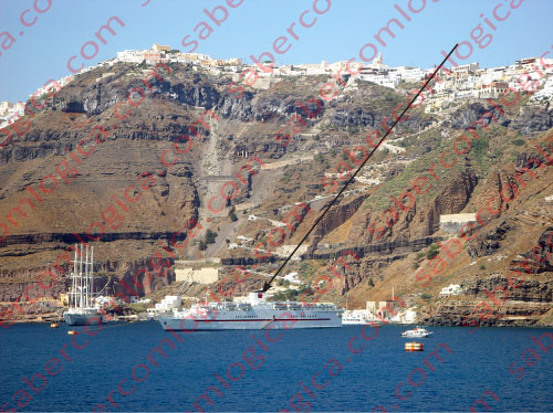
In order to understand this concept of image pixels and screen pixels, we are going to analyze the image in Figure 6, a photo taken with 5 Mega pixels of resolution, and in True Color.

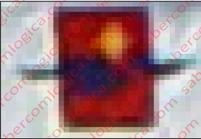
We can clearly see the image’s pixel structure in the screen. But this doesn’t mean that the screen’s pixels have grown. No, that one is fixed, and is as we described before. What happens, is that each pixel of the image takes spans over several pixels of the screen, as we can clearly see in an amplification (not zoom) of the previous figure, displayed in Figure 7.

In order to make this clearer, we prepared this last image:

The stronger white lines represent the squares that compose the image’s pixel structure, and the thinner white lines represent the squares that compose the screen’s pixel structure.

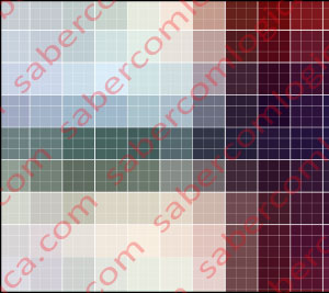
Inside the bigger squares, we can see 9 little squares, which belong to the screen’s pixel structure. Notice that these 9 pixels have the same information, which is the information of the image pixel they contain. This causes a less defined image with a pixel structure similar to the one in  Figure 8, because the image is defined by sets of 9 screen pixels.

We hope that we were able to clarify the difference between the two types of digital image, as well as the differences between the screen’s pixel structure and the pixelized image’s pixel structure.

This last one is dependent on the way the image was captured.

To get the best picture quality on the screen, the ideal solution consists in, once we know the pixel structure of the screen where we want to display it, making its rasterization through the use of a digital image processing program, like Adobe Photoshop for example, so that to each pixel of the monitor, or to each pixel of the printer, corresponds one pixel of the image.

Don’t forget! Always keep the original untouched, should you need to work on it later.

Graphics Card 

Video support can be incorporated into a Motherboard Chip in computers where high video performance is not necessary.

Nowadays it’s becoming more common the incorporation into the CPU (Central Processing Unit) die, of a video chip dedicated to graphics processing, a.k.a. GPU (Graphics Processing Unit), which invalidates our last sentence.

For computers with a powerful CPU, and able to fulfill a demand for high video performances, video processing is done through Graphic Cards connected to slots, having huge transfer rates, and are connected in a point to point fashion with the computer’s Chip responsible for video communications.

The Graphic Cards are printed circuits (much like the Motherboard), that are specifically designed for image processing.

We will avoid referring to any more computer components that we have not yet dealt with. They will all be clarified in the chapter that talks about the Motherboard. For now, we will concentrate on the specific functions of a Graphics Card.

It is the Graphics Cards responsibility to replace or assist the CPU in the complicated and heavy task of creating images that simulate virtual 3D, through complex vector networks (Wireframe) to which, as already mentioned, are added light, texture, color and other elements that contribute to the desired effect, increasing similarity to reality, and to then raster each obtained image into a pixel structure, in order to be displayed on a screen.

Let‘s emphasize the most important components of a high performance graphics card.

A dedicated processor or GPU, which differs from the CPU on the number of processing cores it has. For example, while an Intel Core i7 last generation CPU can have up to 12 cores, the Nvidia GTX Titan’s GPU can have up to 2,688 cores.

This GPU architecture is justified if associated to the complex software developed by its manufacturers, for parallel computing.

In image processing, it’s possible to greatly increase performance through parallel computing, since a huge number of threads can be launched in parallel without competition problems, and contribute to the same final result, the image.

This way, it’s easy to understand how much faster a GPU is than a CPU regarding image processing, and its ability to parallel process.

High Bandwidth, GDDR5 SDRAM, with a much larger bandwidth than DDR3 SDRAM, since its chips are directly integrated into the graphics card (e.g. 384 bits). With specific characteristics, it can achieve transfer rates of nearly 300 GB/s.

The purpose of this paragraph was sensitizing you to the capabilities of the GPU in image processing. As we can see from the described performances, they are irreplaceable when dealing with 3D simulation games or scientific applications in medicine, mathematics, meteorology, astronomy, and other areas, which have higher demands when it comes to image processing.