Routing

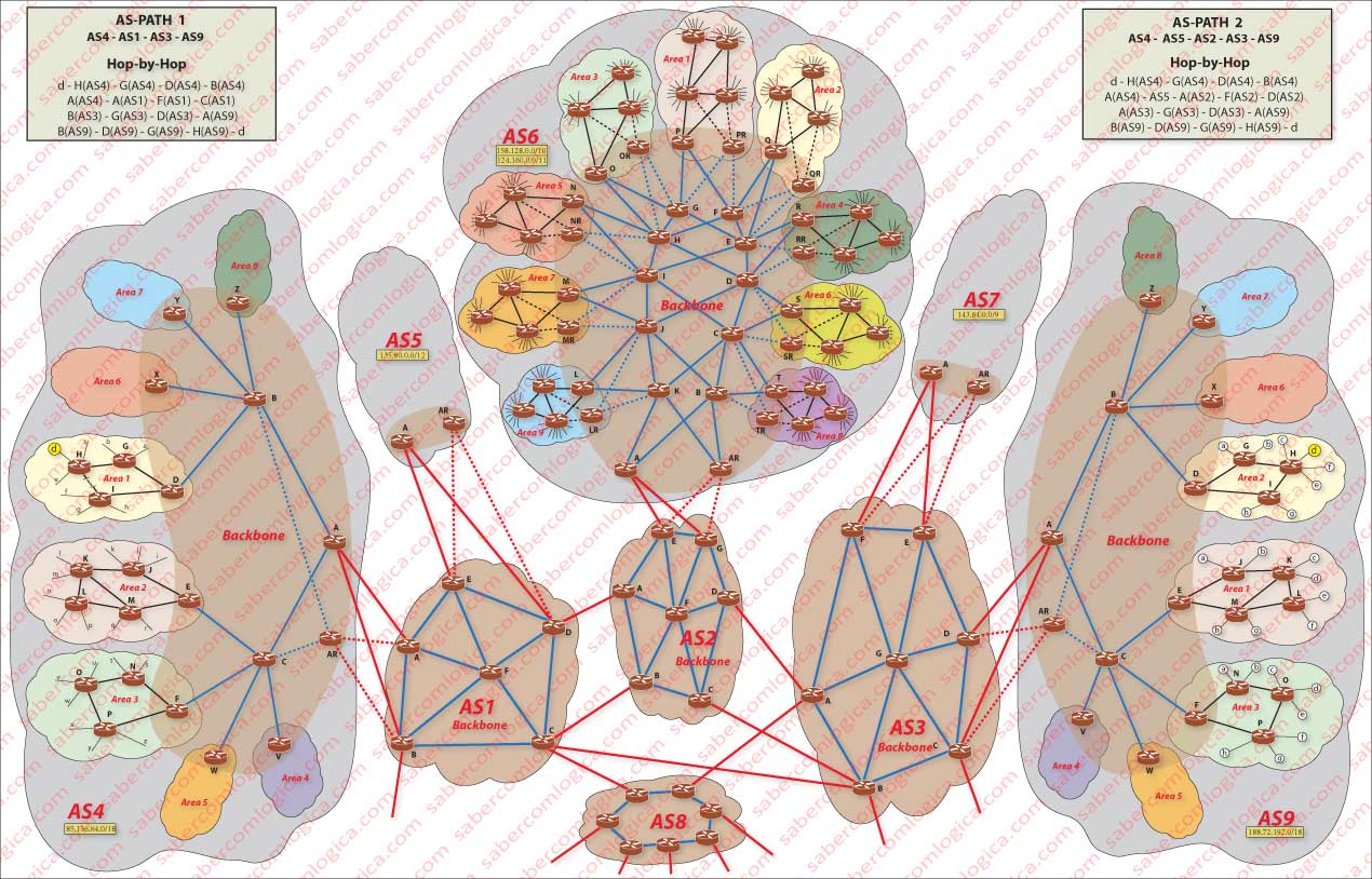
Routing is the determination of the route a packet must follow, router to router, to move from Lisbon to Sydney (e.g.). As we shall see it’s an elaborated process, with many possible algorithms, which we must understand in order to be able to understand all the process as a whole. As graphic support let’s use Figure 1. In order to have it present during all the references you can click or touch in it and open it in another window.

Generic Definitions and References

The cost of a link is the weight that is assigned to a link on the total weight of the route. The cost of a route is the sum of the costs of all the links of the route.

Hop is the route between two routers. The traffic in Internet is made Hop-by-Hop, i.e. from router to router, all the way from source to destination.

The major purpose of routing is to keep routers informed of what is the best way to get somewhere, the one with less cost, and what is the next hop router in that way, so that it can send the packet to it. Internet is a dynamic network, i.e. there are permanent changes of host addresses, new hosts coming, routers that go down, routers that come up, new routers, etc. This means that the knowledge that routing pretends to give to routers about the best way to everywhere, must be permanently recalculated and actualized.

Gateway is the name of an I/O router of a subnet. It’s the door of our home.

An Autonomous System (AS) is a set of routers that are under the same administrative and technical control and running the same protocol. Let’s consider the global network space divided in AS with a reference number on its front. Actually this is the normal representation for them, all AS having a number on the front, which gives them a unique ID – ASn.

Stub subnets, are the subnets where the incoming traffic is intended for them and the outcoming traffic comes from them. They are excluded from this requirement of having a unique ID. We can consider that the subnets represented in Figure 1 with lowercase letters are stub networks, belonging to small organizations or small ISPs, thus getting out of the reference numbering and AS.

Let’s consider two types of routing:

• IGP (Interior Gateway Protocols) , there being used essentially two protocols:
  • RIP (Routing Information Protocol) and
  • OSPF (Open Shortest Path First).
• BGP (Border Gateway Protocol).

Intra-AS Routing

This refers to routing within the Autonomous Systems, where live RIP and OSPF.

RIP (Routing Information Protocol)

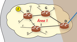
For an easy reading and interpretation we include here a magnification of the  AS4 Area 1 which will be now analyzed, through the Figure 1a.

RIP is a DV Protocol (Distance Vector) that uses the hop count as a cost value. For this is assigned the value 1 to the cost of all the links. So, the best route (lower cost) is the one that has fewer hops. Hop is the route between two routers.

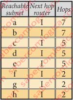
Each router maintains a routing table, the RIP table. In this table are all the attainable subnets, with reference in each case for which is the next hop router for that subnet and the hop number (distance vector) until that subnet is reached, including the hop to the input router (Gateway) of that subnet.

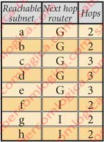
Let’s see how is the RIP table of router D, from Area 1 of AS4, for the various subnets that it can reach, in Figure 2. For this table was assumed that the sub lowercase networks are reached from the nearest router with a single hop and that the link between routers I and H, for having a stroke halted, will have an undefined number of routers along the way.

The RIP tables, which exist in each router on the network are transmitted every 30 seconds for each one to neighbors. Passed 6 periods without transmission, the neighbors assume the router in question is down.

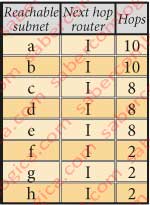
Let’s suppose that there is a problem with the physical link connecting the routers D and G. Router D knows about it and, through the knowledge of its neighbors tables it will recalculate its RIP table to all reachable subnets. Admitting that the number of hops between I and H is 5, then the RIP table of router D will look like in Figure 3.

We admit that the value of 5 hops between I and H is due to the fact that one of the intermediate routers was temporarily down, for reasons of maintenance. When it returned to life, the number of hops between I and H came from 5 to 2. As router H has known about it through its neighbors RIP table it has recalculate its own RIP table. So D did through the knowledge of router H RIP table. The RIP table of D has the shape of Figure 4.

And when the affected link between routers D and G will be repaired, the RIP table of router D will be again the one in Figure 2.

These changes can happen each 30 seconds, reason by which sometimes two packages of the same file follow such different paths to arrive at its destination.

In a DV protocol, each time a node detects changes in the vector of distances, provided that the minimum value of the path to any network is changed it communicates the fact to its neighbor, and so on.

But RIP accepts a maximum of 15 hops, a limitation that restricts its use to small AS.

For this reason, OSPF protocol was conceived. It is the successor to RIP, although RIP still continues to be widely used. In the case of Figure 1, due to the AS admitted dimensions, the Protocol considered is OSPF.

OSPF (Open Shortest Path First)

The Open (open comes from open source) Shortest Path First, was designed to be the successor of RIP. So being, it is not difficult to understand that it has great technological improvements regarding this one.

OSPF is a LS (Link State) Protocol.

In this type of Protocol, as each node knows the identity and weight of each one of its links, it sends a broadcast to all nodes of the network about its link state.

This way it is possible for any node in the network to build a map of the network topology, with identification and weight of all nodes and links. Each node (router) maintains a copy of LS database (LSDB-Link State Data Base) of the entire network of the AS or of its areas.

This database, containing the total composition of the AS or its areas subnets, has in each entry an interface identifier, a link identifier and a cost.

Then each node implementing SPF algorithm (Dijkstra) that describes how a node, according to Mr DijKstra, calculates the shortest path to all other nodes on the network, builds a table with these values, considering himself as the root of the table.

OSPF allows a tiered system within the same AS. In Figure 1, we can see how this tiering was implemented within the AS. Three independent Areas were created in which the Intra-Area routing involves only those routers that are within this area. Each area is identified by a 32 bit number, usually expressed in the form of 4 decimal numbers dot separated, such as IPv4, but without any possible confusion between the two.

The existence of these autonomous areas requires the existence of an area border router ( D, E, F, V, W, X, Y, Z respectively to the Areas 1, 2, 3, 4, 5, 6, 7, 8 from AS4) which, in conjunction with other routers (C and B) to which the AS4 border router (A) must be added, execute the inter-areas routing within AS4. This set of routers is the AS4 Backbone area, represented by the Brown shadowed area in Figure 1. In conclusion, the AS4 Backbone is represented by the routers A, B, C, D, E, F, V, W, X, Y, Z.

Let’s try a little history to illustrate all this in practical terms. Once again the driver of the car. This time it brings a packet of a client from the ISP FRANCOM for a company of Mafra, client of the ISP PORCOM.

• Somewhere in its path he finds a signalman that tells him the route to other signalman who knows how to get to any client PORCOM (the AS border router).
• When arrived, this signalman indicates to the driver the route to the signalman who knows LISCOM customers, a PORCOM dealer that provides PORCOM customers in Lisbon District (the Area router).
• This last one knows all the best path for the driver to get to Mafra. But as that path is very confuse, going through lots of intersections he sends him through his signalmen friends that he knows will drive him, signalman after signalman, to the client of Mafra.

Of course, the representation of 8 areas is illustrative only. Surely they will be many more.

In OSPF the network administrator can assign weights to each link. The weights are influenced by the bandwidth of the link (the less width the more weight), by the availability of the link, by distance expressed by RTT (Round Trip Time), for the reliability of the link and others. When an administrator wants that packets follow a link preferred to him, he only has to attribute more weight to the other links then to that one. Thus, there may be longer paths (in terms of traveled routers ) with lower costs and the path that has the lowest cost is always the chosen.

OSPF allows load balancing traffic by paths with equal cost. It doesn’t have to be chosen a concrete path as in the RIP. In every moment, each router runs its traffic to any of the routers who lead to the same destination with the same cost.

OSPF introduced security in state messages exchanged between routers, as a way to prevent false routing packets could be sent, allowing only authorized routers to communicate with each other.

For this purpose routers are pre-configured with a shared secret key. In the packages that the routers exchange among them are included hash messages built with this key, thus allowing the recipient to confirm the authenticity of the sender.

OSPF supports CIDR and therefore addresses with sub network masks of variable length.

We will now begin our journey outside the AS. But before we go, we want to let you know that the BGP protocol that we’ll analyze there is used in the Intra SA Routing in its iBGP version, but only in the AS Backbone Areas. We’ll understand this a lot better during the Case study analysis.

Inter-AS Routing

ISP Hierarchy

ISPs (Internet Service Provider) are divided into hierarchical levels. ISP access, typically below 3 levels of ISP, can be business networks, campuses or ISPs that provide exclusively direct service to end customers and are served by top-tier ISPs. This access to end customers can also be done directly by top-tier ISPs.

The 1st level ISPs, are the AS that constitute the backbone layer of the Internet . They are in small number, in the order of dozens, they have international coverage, each one being directly tied to all the others and connected to several 2nd level ISPs. Extraordinarily these can provide services to government organizations or enterprises of very large size.

The 2nd level ISPs use the services of 1st level ones, being connected to one or more of them, and some can even be connected to each other. They provide services to 3rd level ISPs, access ISPs or even end customers. To do this, they can be divided into autonomous Areas within a single AS.

Figure 1 represents as 1st level ISP those which only provide backbone services. All 2nd level ISP, regardless of whether they can be linked between them, also are connected to one or more 1st level ISP.

The 2nd level ISP, represented by grey colored spaces, divide their services by autonomous areas, represented by multi colored spaces, creating a backbone area of the AS brown shadowed within the grey space that represents that ISP.

These areas act as if they were 3rd level ISP, though they are an integral part of 2nd level ISP, providing services to access ISP, represented by the lowercase letters.

Imagine your Internet provider. If it is a major enterprise it can be one of these. If it is a little enterprise it will probably be an access ISP.

Any of them provides Internet access services at national, regional or local level and even direct to end-users.

In the case of end users who use DSL (Digital Subscriber Line), cable or optical fiber services, the equipment that is placed at our homes is a NAT router, which makes a private network with the computers we link to the switch behind it, connected to its inside interface. The NAT router has another interface to the outside, to which is assigned a DHCP address.

The address of the router interface in the inside (the side of the private network), for example 198.162.1.1, that gives access to the router interface to the outside (the side of Internet), it’s the door of our computers to the public network, what is known as Gateway.

BGP (Border Gateway Protocol)

Since we have just referred the name gateway, here it is again, but now designing something at a higher level than the door of our home. Gateway designates the gate to the way in our out of some autonomous space, which must be crossed by whoever wants to get in or out of that space by a specific path.

For a user connected to an access ISP to be able to find a server in a AS different from the one it belongs to, somewhere in the world, it needs to use routers which communicate through BGP. It is through this Protocol that the various AS make them known to each other.

BGP establishes TCP semi-permanent connections between BGP peers. These connections can be, as shown in Figure 1:

• IBGP (Internal Border Gateway Protocol) internal to an AS, linking several Areas but always within backbone areas, as is the case of the blue lines.
• EBGP (External Border Gateway Protocol) external to any AS, thus linking two AS border routers, as is the case of the red lines.

Semi-permanent connections. What is that?

In fact connections should be permanent, but among the messages that routers exchange according to the Protocol, one of them is the KeepAlive message, which they repeat for an agreed period of time. In the absence of such a message the connection is terminated.

Other types of messages that are exchanged between BGP routers have as purpose to:

• Initiate a TCP connection with a configured BGP peer,
• Update information about each route being advertised to the BGP peer and
• Notify its BGP peer, when a timer expires or when an error occurs, when it goes to idle and the why.

In BGP announced destinations are not addresses but CIDRized prefixes. Each prefix represents a subnet or set of subnets that can be reached through the router announcing those prefixes.

But, in all headers that we have seen so far there was no room for CIDRized addresses, i.e. network address with net mask together. How is it?

And indeed so it is. This address type is the router itself that builds and adds to its routing table. And constructs the table according to the information that it will receive and propagate.

But, in the routing table that we saw there wasn’t also room for that?

The way that we have seen it, there really wasn’t. Let us remember what it was like in the table of  Figure 2 above, where:

• Subnet ID is its CIDR address,
• Next hop is the ID of the next router and
• Cost is the weight for this binding.

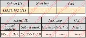
Now let’s look at the same table in Figure 2 below, written otherwise already fairly understandable to the computer when treating CIDR addresses and BGP:

• Network adress and subnet mask describe the network ID. The address 185.35.192.0 with the mask 255.255.192.0 mean the same that 185.35.192.0/18.
• Gateway means the same as next hop, that is, contains the address of the next router interface. Gate to the way.
• Interface indicates the ID of the local interface that should be used to reach the next hop. As we all know, for each Input/Output of the router there is an interface with a specific address.
• Cost indicates the cost associated with the use of the route indicated. Metric is another term that can be associated with, since the network administrator can use it to establish their preferred routes. So being, it has nothing to do with the link cost.

The components of the first table need to be decomposed into the second table in order to be understood by the router. To this table can also be added information such as the AS-PATH (below we will see what this means), links to routes filtering criteria and other.

When a router or host with routing capability is connected to the network it receives from its neighbors the respective routing tables, each one indicating itself as next hop for its table routes. In BGP updates between routers refer to routing tables, being transmitted only when necessary. Link verification regarding neighbors is made by any router through the KeepAlive message.

CIDR addressing gives routers route aggregation capability, i.e. given a set of routes that repeat the same initial bits, router can aggregate all these routes into one to submit the address considering only the bits that repeat themselves and with the due mask.

If through a router the 188.72.(192, 200, 208, 216, 224, 232, 240, 248).0/21 networks are attainable he proceeds immediately to the aggregation of those routes and records in the table as 188.72.192.0/18 for all those routes.

We would like to highlight another property of CIDR addressing. Suppose that one of those routes advertised behind, for example the 188.72.216.0/21 was not part of the network attainable by that route.

Then the router could no longer do the aggregation!

Foregone conclusion. It will do it the same way, because the route to the 188.172.216.0/21 will be part of another announced route, being one BGP over CIDR announced properties that it always opts for the route on which the matching bit number is greater. In this case, despite also being announced at first, as it founds a more specific announcement, it opts for this last one.

Let’s see if we understand how a BGP router on Internet can have knowledge of all possible routes and all existing destinations. If it were not for CIDR, this would give a huge table. But even so, the number of entries in a routing table was in 2010 more than 300,000.