
The bits and the Magnetic fields
How Data is registered
With what we learned about the elements of an Hard Disk Drive (HDD), we can now understand how the information is registered. The information that reaches the HDD to be stored is composed of bits which carry logic states 1 or 0, that correspond to the physical states with or without voltage. The HDD, in order to save those physical states of voltage, has to translate them into magnetic fields.
There is a general tendency to consider that logic state 0 corresponds to a certain magnetic orientation, to which the opposite one will correspond the logic state 1. That would be logic. But it can’t work that way. The HDD isn’t ruled by a clock, simply by platter speed, which can have slight variations, and so can the density along the platter. This would make very difficult, after a log sequence of 0 or 1, telling how many they were or in which position bit x would be. It would be like being in the middle of the desert, without any measuring instrument, and having to know where we are.
It was necessary to introduce flow inversions somewhere in the middle of chains with equal bits. For that reason, it was decided that the information would be stored under the form of magnetic flow inversions. The logic value 1 would be represented by an inversion in the magnetic flow (N→S to S→N and vice-versa) and the logic value 0 would maintain the magnetic flow.
The problem still persisted, though. But this time, limited to the zeros. How would it be possible to define the quantity and position of a long chain of bits during and after a long chain of 0? So the coding methods for bits appear, of which we will describe the more expressive ones, starting with the simpler and going up to the more complex ones.
FM (Frequency Modulation)
This method consists in introducing a flow inversion between each bit, as a clock sign orientation, after which there would be, or not, another inversion to 1 or 0 respectively. It is graphically represented In figure 1 above as well as the table of relations between the bit value and flow behavior. I represents the existence of flow Inversion and N represents Non inversion of flow.
This method spends half the capacity on disk in clock inversions. As we can see on the graphic, each bit is represented by two magnetic fields:
- One inversion to signal the clock .
- Another that informs us if we are facing a 1, with a new invertion, or a 0, keeping the direction of the magnetic field.
In our bit set case – 1 0 0 1 0 0 0 0 1 1 1 1 – we should represent it as – IIININIIININININIIIIIIII – from which result 18 flow Inversions.
The FM coding method was essentially used in simple density floppy disks.
The graphics on figure 1 (below) present an example of FM with perpendicular recording. In its epoch, such technology wasn’t yet available, but we opted by using this type of representation because it is possible to do it in the available space. For this same reason, we will continue to use this type of representation.
MFM (Modified Frequency Modulation)
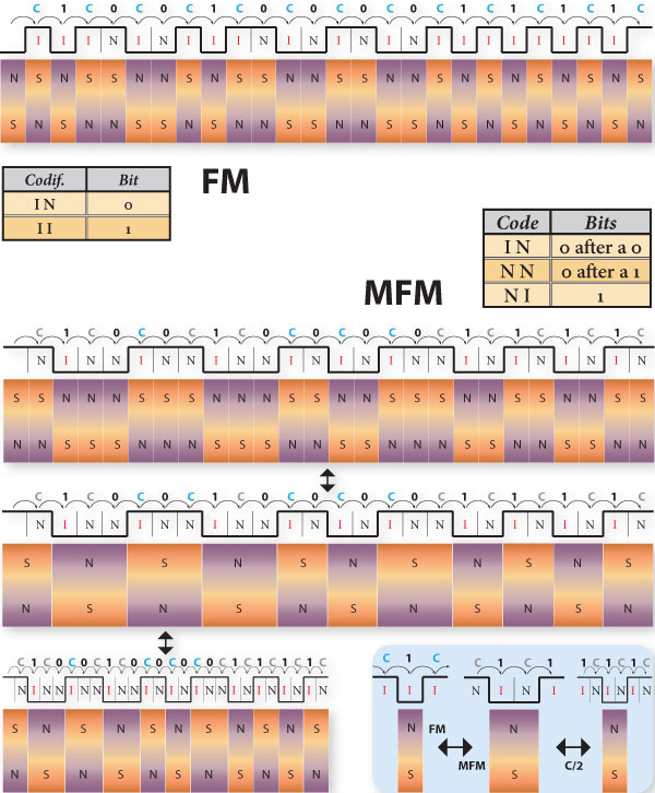
This method is an improvement of the previous FM method.
Attending to the fact that platter density is defined by how many flow inversions it supports, the main goal is to reduce the number of inversions needed to represent the same set of bits, maintaining however the distancing between flow inversions within the minimum value considered to the FM method we’ve just seen, i.e. maintaining the magnetic field size.
This way, instead of inserting a flow inversion between any two bits, this method involves integrating a flow inversion between two consecutive 0. Let’s see it graphically represented on figure 1 (below).
Let’s focus only on flow inversions. Note that the distance between flow inversions in this graphic is now, at least, twice as the graphic before.
The clock signal is still happening in the middle of every small field, though now it is only represented by an inversion between two 0. Since fields of similar orientation have additive properties, the result is the 2nd line of figure 1 (below).
We can then reduce the clock value in half, thus reducing the smaller fields dimension to a value never smaller than the minimum between flow inversions, defined in the first graphic for FM. The result is the 3rd line of the figure 1 (below).
The coding of each bit is described in the annexed table. We can represent in magnetic record, the same amount of bits in half the space then previously with FM.
In our bit set case – 1 0 0 1 0 0 0 0 1 1 1 1 – we should represent it as – NINNINNINNINININNINININI – from which result 10 flow Inversions.
In this case, determining the clock signal isn’t as clear as in the FM case.
It’s the HDD logic board function to code/decode the digital bits into analogue signals (magnetic) and vice-versa. Its determination has to be done considering the bits before and after the reading, or yet, the magnetic fields behavior after reading or while writing.
The MFM method originated the double density floppy disk. It was quickly replaced in the HDD.
RLL (Run Length Limited).
Run, designates the set of magnetic zeros, i. e., non flow inversions (N) in a row.
Length, designates the minimum number N (non flow inversions) to be used in a row.
Limited, represents the maximum number N (non flow inversions) to be used in a row
RLL has two defining parameters: a and b, a being Length and b being Limited, presenting itself under the formula RLL(a,b).
We shouldn’t consider it a method, but a series of methods that depends on the considered parameters, varying from parameter to parameter. Let us analyze the codes RLL(1,7) and RLL(2,7)
RLL(2,7)
This method, which means representations with Runs with a minimum of 2 and a maximum of 7 non flow inversions (N), which is represented on figure 2 (above), is quite more elaborate than the ones before, considering the coding by bit groups instead of the coding of each individual bit. The groups of bits and their representation follow the pattern shown in the same figure for RLL(2,7).
This table was found based on the following principles:
- Each flow inversion is followed at least by 2 non inversions.
- Each group should initiate with a number smaller or equal to 4 non inversions.
- Each group should end always with a number smaller or equal to 3 non flow inversions.
This method uses blocs of 2, 3 and 4 bits, always represented by 4, 6 or 8 magnetic fields. With the groups represented in the annexed table, it is possible to unequivocally represent one, and only one, group of bits, respecting the magnetic field sequence of the earlier premises and represent all possible bit sequences.
In our bit set case – 1 0 0 1 0 0 0 0 1 1 1 1 – -we should represent it as – 1 0 – 0 1 0 – 0 0 0 – 1 1 – 1 1 – to which it will correspond – NINN – INNINN – NNNINN – INNN – INNN or NINNINNINNNNNINNINNNINNN, from which will result minimum Runs of 2 and maximum of 5, in this case, respecting the minimum and maximum defined.
For the group of bits we’re representing, we can see that, in the FM case we needed 18 flow Inversions, in the MFM case 10 flow Inversions and in the RLL(2,7) case 6 flow Inversions.
Since what matters to us is the flow inversion density, we can see by inversion counting that this method has 3 times less inversions than the FM, i. e., for the same clock, the distance between flow inversions is three times from the initially considered and supported by our hardware. This can be verified in the 2nd line of figure 2 (above), after the additive property in the adjacent magnetic fields with the same direction is applied. Let’s divide the clock sign by 3 so we have our initial distance between flows, without however decreasing the size of the fields that define that distance, resulting in line 3 of figure 2 (above). This way, without suffering any reduction of the magnetic fields, we can multiply by 3 the bit density representable in the same space in relation to FM.
RLL(1,7)
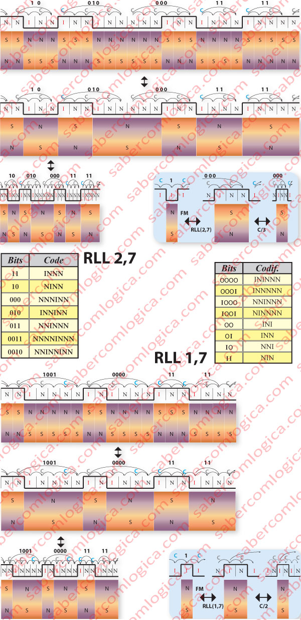
This method, which represents Runs with a minimum of 1 and a maximum of 7 of non flow inversions (N), shown in figure 2 (below), codes groups of 2 or 4 bits in groups of 3 or 6 magnetic bits.
Notice that this method represents each 2 bits with 3 magnetic flow combinations, contrary to all the previous ones, which represented 2 bits with 4 magnetic combinations. Therefore it won’t be needed as much magnetic bits to represent the same number of logic bits.
The logic board, when coding a group of bits, takes 2 and looks at the 2 that follow to check if they fit in any possible combination. If so, it uses the combination of 4, if not, it uses the combination of 2. While decoding, it does the same with groups of 3 magnetic bits.
The annexed table referring to the bit grouping an its coding used by this RLL was established by the following set of rule, considering that to 1 corresponds an Inversion (I) and to 0 a Non inversion (N):
- (x,y) binary converts in (NOT x, x AND y, NOT y) in magnetic bits.
- (x,0,0,y) binary converts in (NOT x, x AND y, NOT y, 0, 0, 0) in magnetic bits.
In our bit set case – 1 0 0 1 0 0 0 0 1 1 1 1 – we should represent it as – 1 0 0 1 – 0 0 0 0 – 1 1 – 1 1 – to which it will correspond – NINNNN – ININNN – NIN – NIN or NINNNNININNNNINNIN, from which result minimum Runs of 1 and maximum Runs of 4, in this case. In the RLL(1,7) we verify that we need 5 flow Inversions
We can verify that the distance between flow inversions, after the field association is applied, is twice as the one we have for FM, considering the maximum concentration supported by the HDD, according to line 2 of the figure 2 (above). This way, we can reduce the clock value in half, maintaining the regular distance between magnetic field inversions. This results in line 3 of the figure 2 (below).
In Figure 3 we are comparing the final graphs of the different types of coding, so being possible to see the evolution of the space occupied in the disk to represent the same number of bits in the different methods.
The increasing in bit density magnetically represented in the same space we have been working with, is the result of the applied methods of coding alone.
This is possible with digital to analog (magnetic fields) translation software and vice-versa. And with this we already reduced by 1/3 comparing with the first method we talked about.
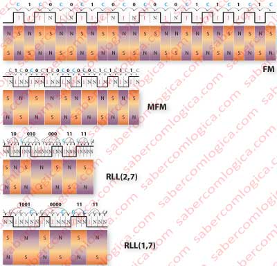
In the RLL case, coding groups of bits rendered unnecessary the introduction of marker bits that were in use in the previous ones. It however made logic boards more important, since they read, interpret and decode analogical signs.
As we can see, the density rises as much as the clock can be reduced, which depends on the minimum value of 0 in a row (RLL(2,7)) and the more the combinations increase, representing as much bits as possible with the least amount of magnetic bits (RLL(1,7)).
The best case scenario in each of the possibilities can be seen on RLL(2,7) and on RLL(1,7). In this case, the first one wins.
However, with the available reading processes, Runs bigger than 7 were not recommended, risking losing the head alignment and thus, their sync, losing track of which bit they were on.
The reading was usually made by peaks, i. e., the heads would identify the flow inversion by reading the areas where the fields would reach their maximum. In terms of hardware, its evolution, as we already observed, led to really small magnetic fields, with very little intensity and very hard to read.
With the increase in density, the reading process by peaks became ineffective, since the difference between the various reading points was so small and so close, the heads couldn’t tell where one ended and another started, and readings being sometimes even disturbed by noise caused by field proximity.
Thus a new method for reading came along, based not on peaks, but in a sampling of several values done during the wave evolution, of which an average by likelihood would be calculated.
PRML (Partial Response Maximum Likelihood)
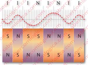
This is precisely what was described earlier and we’ll attempt to illustrate it in figure 4.
This reading method forced the development of extremely complex logic boards that, with a huge sensitivity to any variation, obtain the “partial answers” that cause the determination through flow variation, for the effect using algorithms of great complexity, calculating them by likelihood.
This method was refined by EPRML (Extended Partial Response Maximum Likelihood). O EPRML works in a very similar way to the PRML, however reaching significantly higher performances at a more complex processor and more complex algorithms.
With such an improvement in reading and interpreting the signs, with enhancements in perpendicular recording in signal quality, it was possible to obtain greater accuracy in determining the readings, which allowed extending the maximum number of consecutive zeros without the risk of the head losing track of itself
This way, with RLL coding with parameters which maximum can reach between 16 and 20 consecutive zeros, also increasing the minimum of consecutive zeros, it was possible to obtain tables representing much more elaborate bit groups, allowing huge reductions in the necessary magnetic bits to represent a specific number of digital bits. All based on the evolution of Logic Boards.